How to Calculate an Interest Payment in Excel: 7 Easy Steps

Excel can calculate the interest portion of a loan payment faster than you can say “variable APR.”
The trick is knowing which interest you mean. Are you trying to find the interest in your
first payment? The interest in payment #37? Or the total interest
you’ll pay if you keep making minimum payments until the sun burns out (aka a 30-year mortgage)?

This guide walks you through a clean, reliable way to calculate an interest payment in Excel
using the right functions (especially IPMT and PMT), plus a quick
amortization setup for sanity-checking your numbers. No finance degree requiredjust a willingness
to let Excel do the math while you take the credit.

What “interest payment” means (so Excel doesn’t roast you later)

For an amortizing loan (mortgage, car loan, most personal loans), your periodic payment usually includes:
interest (the lender’s fee for letting you borrow money) and principal
(paying back what you borrowed). Early payments are typically heavier on interest; later payments shift toward principal.

Excel can calculate the interest portion for any period as long as the payment amount is constant and the interest rate is constant.
If your loan changes rates, your spreadsheet can still handle ityou’ll just need a slightly more “grown-up” setup (we’ll get there).

Step 1: Gather your loan inputs (and put them in cells like a responsible adult)

Before you write formulas, collect the basics. Put them in a tidy “Inputs” area so you can update the loan later without rewriting everything.
Here’s a practical set:

• Loan amount (PV): the amount you borrow (present value)
• Annual interest rate (APR): e.g., 6% (as 0.06 in Excel)
• Loan term: in years or months
• Payments per year: 12 for monthly, 26 for biweekly, 52 for weekly, etc.
• Payment timing: end of period (most loans) vs. beginning (some leases/annuities)

Pro tip: Name your input cells (Formulas > Define Name). “APR” is easier to read than “$B$2.”
It’s also easier to debug when Excel starts acting like it’s on caffeine.

Example inputs

Let’s use a realistic scenario you can copy:

• Loan amount (PV): $250,000
• APR: 6%
• Term: 30 years
• Payments per year: 12 (monthly)
• We want: interest payment in month 1 (and any month after)

Step 2: Convert the annual interest rate to a per-period rate (don’t skip this)

Excel’s loan functions expect the interest rate per period. If your APR is annual and payments are monthly,
the periodic rate is typically:

Periodic rate = Annual rate / Payments per year

In Excel, if APR is in B2 and payments per year is in B5:

For 6% APR and monthly payments: 0.06/12 = 0.005 per month (0.5%).

APR vs. effective rate (quick reality check)

Most consumer loan calculators treat APR divided by 12 as the monthly rate for these functions.
If your lender uses a different compounding convention, you may need an effective-rate conversion.
But for most standard fixed-rate loans, dividing by payments per year matches common amortization logic.

Step 3: Calculate the total periodic payment with PMT

The PMT function returns the regular payment amount for a loan with constant payments and a constant rate.
It’s the foundation for everything else.

PMT syntax (human version)

PMT(rate, nper, pv, [fv], [type])

• rate: interest rate per period (monthly rate if monthly payments)
• nper: total number of payment periods (years × payments per year)
• pv: present value (loan amount)
• fv (optional): future value (usually 0 for a fully paid loan)
• type (optional): 0 = end of period (default), 1 = beginning

PMT example formula

Suppose:
APR in B2,
TermYears in B3,
PV in B1,
PaymentsPerYear in B5.

Notice the negative sign on B1. Excel financial functions follow cash-flow signs:
money you receive vs. money you pay. Using -B1 typically returns a positive payment amount,
which is friendlier for humans who prefer positive numbers and positive vibes.

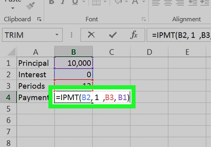
Step 4: Use IPMT to calculate the interest payment for a specific period

Here’s the star of the show: IPMT. It returns the interest portion of the payment in a given period.
If you want the interest paid in month 1 (or month 180), this is your tool.

IPMT syntax (still human)

IPMT(rate, per, nper, pv, [fv], [type])

• rate: interest rate per period
• per: the payment period you care about (1 through nper)
• nper: total number of periods
• pv: present value (loan amount)
• type: 0 end of period, 1 beginning

IPMT example: interest in month 1

With the same inputs as above, month 1 interest:

Want month 37 interest? Change 1 to 37.
Excel won’t complainunless you accidentally type 3700, in which case it will silently judge you with #NUM!.

Make it dynamic (best practice)

Put your desired period number in a cell (say B7) and reference it:

Now you can type any period into B7 and instantly see that period’s interest payment. It’s like a remote control for debt.

Step 5: Sanity-check with the simple formula (because trust is good and verification is better)

For period 1, the interest portion is basically:

Interest = Beginning Balance × Periodic Rate

In month 1, the beginning balance is the original loan amount. So for our example:
$250,000 × 0.005 = $1,250.
That means your first payment’s interest should be about $1,250 (give or take rounding conventions).

This quick check is especially useful if you’re new to Excel IPMT and want confidence that your spreadsheet isn’t inventing numbers.
If IPMT gives you something wildly different, the usual culprit is a mismatch between annual vs. monthly rate, or years vs. months.

Step 6: Build a mini amortization schedule (the easiest way to see what’s happening)

If you want interest payments for multiple periods, an amortization table is the cleanest view.
And yes, it also makes you look like a spreadsheet wizard in meetings.

Set up columns

Create a table with these headers:

Example formulas (assuming row 2 is period 1)

Let’s assume your inputs are:
B1=PV, B2=APR, B3=TermYears, B5=PaymentsPerYear.
In your schedule:
A2=Period, B2=BeginningBalance, etc. (use your own cell references as needed).

• Period (A2): =1 then fill down =A2+1
• Beginning Balance (B2): =$B$1
• Payment (C2): =PMT($B$2/$B$5, $B$3*$B$5, -$B$1)
• Interest (D2): =IPMT($B$2/$B$5, A2, $B$3*$B$5, -$B$1)
• Principal (E2): =C2-D2
• Ending Balance (F2): =B2-E2

For period 2 (row 3), set Beginning Balance to the prior ending balance:
=F2 and fill down.
Your interest portion will gradually drop as the balance shrinksbecause the lender can only charge interest on money you still owe.

Want the principal portion directly?

Excel has PPMT for that (principal payment for a period). It pairs naturally with IPMT.
But you can always calculate principal as Payment - Interest like above.

Step 7: Handle real-life wrinkles (because loans love drama)

1) Payments at the beginning of the period

Some loans/leases assume you pay at the beginning of each period. In that case, use type=1 in both PMT and IPMT.
Example:

2) Extra payments (a.k.a. “how to save thousands without feeling joyless”)

If you make extra principal payments, the simple IPMT approach (constant payment assumptions) won’t match perfectly,
because your balance drops faster than the standard schedule.

Solution: use the amortization table approach and subtract extra principal in your ending balance formula.
Add a column like Extra Principal and update:

3) Variable interest rates

If the rate changes over time (adjustable-rate loans), IPMT with a single constant rate is not enough.
Use a schedule where each row has its own periodic rate and calculate interest as:

Then you can still compute principal as Payment - Interest and keep the table honest.

4) Rounding differences

Lenders often round at the cent level each period, which can cause tiny differences by the last payment.
In Excel, that’s normal. Use rounding strategically (e.g., ROUND(value,2)) if you need to match a lender statement.

Common mistakes (and how to fix them fast)

Your interest is negative

That’s usually a sign convention issue. Excel might be returning cash flows (payments) as negatives.
If you want a positive-looking interest payment for reporting, wrap with:

You used years in one place and months in another

If payments are monthly, everything must be monthly:
rate per month, number of months, and the “period” measured in months.
Mixed units are the #1 reason Excel interest formulas go off the rails.

#NUM! error in IPMT

This often means the period (per) is less than 1 or greater than nper,
or that inputs are inconsistent (like a negative loan amount plus a negative PV sign).
Check per and confirm your PV and payment sign choices.

Quick FAQ: Excel interest payment calculations

Is IPMT only for loans?

IPMT is designed for scenarios with constant payments and a constant interest rate over fixed periods.
It’s commonly used for loans, but it can also apply to other annuity-style calculations that fit those assumptions.

What’s the difference between PMT, IPMT, and PPMT?

• PMT: total payment each period
• IPMT: interest portion of that payment for a given period
• PPMT: principal portion for a given period

Can Excel calculate total interest paid over the loan?

Yes. The simplest approach is building an amortization table and summing the Interest column.
Or, if you’re using dynamic array functions, you can generate a full schedule and sum it in one go.

Conclusion

If you want to calculate an interest payment in Excel cleanly, remember the flow:
convert your rate to the right period, calculate the payment with PMT, and pull the interest portion with IPMT.
Then sanity-check with “balance × periodic rate,” and build a small amortization schedule when the real world gets messy
(extra payments, rate changes, rounding quirks).

Once you’ve got this setup, you’re not just calculating interestyou’re building a spreadsheet that explains your loan like a story:
what you owe, what you pay, where the money goes, and how fast the balance actually falls. That’s powerful.
Also, it’s a great way to win arguments with calculators on the internet.

Field Notes: Practical Experiences That Make Excel Interest Calculations Way Easier (and Less Annoying)

The formulas are the easy part. The hard part is everything around them: assumptions, inputs, formatting, and the weird ways humans
accidentally sabotage spreadsheets. Here are the most useful “experience-based” habits that make interest calculations in Excel feel
effortless instead of cursed.

1) Build an “Inputs” box and never type numbers into formulas

If you hardcode 0.06/12 into ten formulas, you’ve created ten opportunities to forget where you did it.
Put APR, term, and payments-per-year into cells and reference them. Your future self will thank youand your teammates will stop
sending you passive-aggressive messages like “Which cell do I change to update the rate?”

2) Decide your sign convention once (then stick to it like it’s a family recipe)

Excel’s financial functions care about cash flow direction. The easiest pattern for loan spreadsheets is:
PV as positive in the input cell, then use -PV inside PMT/IPMT so results come out positive.
If you switch conventions mid-sheet, you’ll get negative interest payments and a strong urge to blame Excel.
(Excel is innocent. Mostly.)

3) Make the period number a cell, not a thought

If your interest formula is =IPMT(rate, 37, ...), you’ve trapped the period inside the formula.
Put the period in a cellsay PeriodWantedthen your spreadsheet becomes interactive. This is especially handy
for loan reviews: “What’s the interest in month 12?” becomes typing 12, not editing formulas and praying you didn’t break anything.

4) Always run the “balance × rate” gut check

IPMT is reliable, but your inputs might not be. For period 1, interest should be roughly loan amount × periodic rate.
If it isn’t, you’ve likely mixed monthly vs. yearly terms. This single check catches more spreadsheet bugs than any fancy auditing tool,
and it takes about three secondsless time than it takes Excel to autosave when you’re in a hurry.

5) Use an amortization table whenever money changes midstream

Extra payments, skipped payments, changing ratesthese are the “plot twists” that break constant-payment assumptions.
When the loan is no longer a perfectly steady machine, switch to a schedule-based approach:
compute interest as BeginningBalance * PeriodicRate each row. It’s transparent, it matches reality better,
and it gives you a column you can sum for total interest. Plus, it makes your spreadsheet feel less like magic and more like math.

6) Format for humans: show cents, label periods, and add notes

People don’t trust spreadsheets they can’t read. Use currency formatting, two decimals, and clear labels like “Monthly Rate” and “Total Months.”
Add a short note under your inputs: “Rate is APR; monthly rate = APR/12.” That tiny sentence prevents a surprising number of
“Why are my payments different than my lender?” emails.

7) Expect tiny rounding differencesand don’t start a spreadsheet war over pennies

If your lender rounds every month and your spreadsheet rounds only at the end, totals can differ by a few cents (sometimes a few dollars over decades).
If you need to match statements precisely, round each period’s interest and principal to cents before carrying balances forward.
Otherwise, accept that spreadsheets and lenders don’t always round the same wayand that’s okay. Your loan will still be expensive either way.

Bottom line: Excel makes interest calculations easy, but your spreadsheet design makes them reliable.
Get the structure right once, and you’ll reuse it for mortgages, car loans, student loans, business debt schedulesbasically anything
that involves money leaving your account on purpose.